Master thesis
Approximate
optimization algorithms of
Quadratic Assignment Problem (QAP)
AGH, Faculty of
Automatics and Robotics Engineering, Kraków 2000
|
|
||||||||||||||||||||||||||||||||||||||||||||||||||||||||||||||||||||||||||||||||||||||||||||||||||||
|
|
||||||||||||||||||||||||||||||||||||||||||||||||||||||||||||||||||||||||||||||||||||||||||||||||||||
|
|
||||||||||||||||||||||||||||||||||||||||||||||||||||||||||||||||||||||||||||||||||||||||||||||||||||
|
1.1. General description of the
problem The problem of assigning tasks to resources with a quadratic
quality index QAP (Quadratic Assignment Problem) belongs to the NP-difficult
problems of combinatorial optimization. This problem occurs in numerous
practical issues in such areas as: economics, ergonomics, electronics,
architecture, information technology, etc. For the first time, the QAP
problem was formulated by Koopmans and Beckman [5] for economic applications.
The QAP problem is a generalization of the linear AP (Assignment Problem)
that belongs to the class P - polynomial problems. It is defined as follows. The data are n2
coefficients of costs of assigning tasks to resources Cij and n4 coefficients
of connections Dijkl:
One
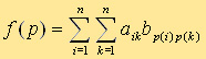
should find the solution
Equation 1. Objective function - general notation. |
||||||||||||||||||||||||||||||||||||||||||||||||||||||||||||||||||||||||||||||||||||||||||||||||||||
|
with limitations:
Decision variable xij = 1
if task or object j is assigned to resource or item i (i,j = 1,.......,n) and
xij = 0 otherwise. In most applications, the cost factors
dijkl can be expressed as the product of the elements of two
matrices A and B:
Equation 3. Cost coefficients where
A - matrix of distances between i and
k positions of objects B - matrix of relations between
objects j and l where
i,k,j,l = 1,2,....,n They are non-negative square nxn
matrices with zero elements on the main diagonal. In this case, the problem
Objective function can be written as
Equation 4. Objective function - matrix notation. Often, in order to shorten the
notation of the problem and simplify the presentation of solving methods, the
solution of the allocation problem is formalized in the form of permutations p = [p (1), p (2), .........., p (n)]
with the set of n prime natural numbers. The problem model, equations 1-4, can
then be written as follows:
Equation 5. Objective function - notation by permutation. where p (i) is
the number of the task or object assigned to the resource or item i, P is the
set of permutations on the set of natural numbers N =
{1,2,.............,n}. QAP optimization methods, like any
other NP-difficult problem can be divided into two main groups: • exact methods (giving the optimal
solution) useful for effective solution of the problem when its dimension n
<20, • approximate methods, more or less
complex, giving a suboptimal solution. They are the only computationally
efficient methods for n> 20. In the next part, the QAP solution
will be presented in the form of permutations p = [p (1), p (2), ............., p
(n)] and the linear component of the objective function(matrix C) was
omitted.
|
||||||||||||||||||||||||||||||||||||||||||||||||||||||||||||||||||||||||||||||||||||||||||||||||||||
|
There are a large number of exact methods. They can
be divided into two groups. The first one is based on the Branch and Bound
Method, while the second one uses various types of linearization of the
objective function. In the first subgroup, simple assignment methods and
double assignment methods can be distinguished. The methods of simple
assignment boil down to the assignment of one element of the (unallocated)
set of tasks, to one element of the resource set, at each stage of the
calculations, until all assignments are exhausted. The group of these methods includes methods that use
QAP decomposition. In this case, the matrices A and B are reduced and the
objective function is decomposed into a linear function and a reduced
quadratic function. Typical representatives of this approach are the
algorithms of Roucairol [9] and Christofides-Mingozzi and Toth [2]. Since the Roucairol algorithm solves relatively
large problems in a user-acceptable time, it can be used to test
approximation algorithms. The algorithm is described below. C. Roucairol presents the objective function as a
sum of a linear function and a reduced quadratic function. This decomposition
makes it possible to easily find both the lower and upper limits of the
optimal solution. Then, using the standard Branch and Bound method approach,
a solution tree is constructed and an intermediate solution review is
performed. The basic steps of this method are shown below for the following
form of the objective function:
Equation 6. Objective function - notation without the linear
component. Phase
1 of the algorithm:
reduction of matrices A and B. M '= [m'ij
] = [mij - ai - bj] is a matrix with non-negative elements and contains at
least one zero in each row and column. 1)
Standard
"row-column" method, known from applications in the Hungarian
algorithm for the AP problem and in the Little (et al.) Algorithm for TSP -
Traveling Salesman Problem. 2)
The
method called "maximal element first" consists in finding the
maximal element of the matrix M:
The maximum element is reduced first.
For this, we are looking for the minimum element in the line i* :
minimum element in column j* :
if now
then we reduce the elements of the
line i* by the value of mi*l
and substitute |
||||||||||||||||||||||||||||||||||||||||||||||||||||||||||||||||||||||||||||||||||||||||||||||||||||
|
ai*
= mi*l , b1 =
0 , and when
then we reduce the elements of column
j * by the value mkj*
and substitute bj* =
mkj* , ak = 0. This procedure successively leads to
obtaining the reduced matrix M'. Reduction
of the QAP problem Let A’ = [a’ik] be the reduced matrix of A., where a’ik = aik
- ai - bk; ai , bk , aik
³ 0 and the matrix B’ = [b’jl] is the reduced matrix of the matrix B,
where b’jl = bjl
- a’j - b’l;
a’j , b’l , bjl ³ 0. The reduced QAP problem is a problem
with the following objective function:
By developing this formula, we prove
the relationship between the original problem and the reduced problem:
where gamma
is a constant defined as the relation:
K(p) is an objective function of an AP
problem of the form
elements of the matrix K = [kij]
are defined by the relation:
Then we calculate the lower and upper
bounds of the optimal solution. Lower
bound Since the reduced matrices A', B' are
non-negative matrices, so
hence
in particular
So you can see that the lower bound of
the function f(p) is
Where
Upper
bound Let p * be the desired solution to the
original problem, i.e.
It is not difficult to compute f (p)
if we know
Because
Ultimately we get
and f '(p) here represents the
difference between the lower and upper bounds. So the implication is right:
Phase
2 of the algorithm:
Solution Tree Intermediate Review Procedure. The optimal solution (assignment) is searched for in
the solution tree in a similar way to Little's Branch and Bound algorithm for
the TSP problem. The double assignment methods were developed in the
works of Land [6], Garett and Plyter [4] and Pierce and Growston [8]. They
come down to the simultaneous allocation of a pair of elements (tasks) (i, k)
to a fixed pair of distributions (resources) (j, l). The QAP problem is
transformed into the AP problem with a cost matrix mm where m
= n (n-1) / 2. The standard technique of the Branch and Bound method is then applied. The second subgroup of strict methods are
linearization methods. These methods transform the quadratic problem into an
equivalent integer linear problem with additional variables and constraints. The Lawler approach [7] is typical for this group of
methods. A QAP problem having n2 xij variables is
linearized by additionally introducing n4 yijkl
variables, where yijkl = xijxkl. The
obtained linear model has n4 + n2 variables yijkl
and xij , and 2n4 + 2n constraints and has the
following form:
with restrictions
A significant disadvantage of
linearization methods is a significant increase in the number of variables
and constraints, which in the case of large sizes of problems significantly
extends the calculation time. When the problem dimension is n> 10, these
algorithms are practically useless.
|
||||||||||||||||||||||||||||||||||||||||||||||||||||||||||||||||||||||||||||||||||||||||||||||||||||
|
• Construction methods • Iterative methods of correcting the
solution
In the first case, the solution is constructed in
such a way that the execution of one iteration of the procedure consists in
determining the value of one component of the solution. Most often, the acceptable
solution is determined using the greedy rule, list scheduling and also by
drawing lots. In the last case, the order of the elements from the set N in
the permutation p is determined by a random number generator. The most
popular of the inaugural methods is the BEST_MATCH procedure, which has been
used by many QAP researchers to generate an initial solution. The basis of
this procedure is the process of assigning the most related (large flow of
materials, parts, patients, large number of connections, etc.) objects
(industrial plants, machines, clinics, modules, etc.) to key items (e.g.
central items).
Step 1. For j = 1, 2, .............,n calculate values
Ordering
the indices j in the order of the non-increasing values of BBj, create the
vector BB.
Line up
the indices and in order of non-decreasing AAi values, create the vector AA. |
||||||||||||||||||||||||||||||||||||||||||||||||||||||||||||||||||||||||||||||||||||||||||||||||||||
|
|
||||||||||||||||||||||||||||||||||||||||||||||||||||||||||||||||||||||||||||||||||||||||||||||||||||
|
Iterative correction methods consist in searching,
in each iteration, for a solution better than the successor, where the best
known solution is the successor. The most popular and effective are the
methods of local optimization, in the scope of which the most frequently
sought solution is better in the vicinity of the successor obtained by
changing the position of two or three elements of the successor, whereby
individual authors propose different rules for changing the position of
elements in the permutation and different rules determining the order of
quality checking solutions from the environment. A representative example of
generating solutions from the successor's environment by changing the
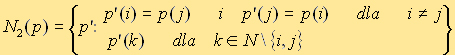
position of two elements of the permutation is the Heider algorithm. If the
successor is a permutation p, then the permutations p' belonging to the
environment of the successor N(p) are defined as follows:
The algorithm systematically checks up to n (n-1)/2
(because |N2(p)| = n(n-1)/2) solutions from the successor's environment in
the order determined arbitrarily or determined by the selected rule. Checking
the solutions from the successor's environment is carried out until the first
solution better than the successor is received, which becomes the new
successor, and the search process is continued in the vicinity of the new
successor. If the algorithm does not find a better solution in the entire
environment of the successor, the successor is the locally optimal solution
and the search process ends. The cost of calculating the value of the
objective function of solutions p' belonging to the environment N2(p) is
reduced if only the difference of the value of the objective function of the
successor p and p' is computed:
If df>0, then the permutation of p' is a better
solution than the successor of p. The calculation of the increment of df
requires the performance of (2n-2) multiplication and (5n-4) addition
operations. Hence, the Heider algorithm is considered by many authors to be
the most effective double change algorithm. This
work focuses on the Tabu Search procedure, which is also based on the double
change method and is described in detail in point 1.4. |
||||||||||||||||||||||||||||||||||||||||||||||||||||||||||||||||||||||||||||||||||||||||||||||||||||
|
|
||||||||||||||||||||||||||||||||||||||||||||||||||||||||||||||||||||||||||||||||||||||||||||||||||||
|
Create a boot solution using the construction
procedure. Substitute:
K - number
of iterations, T - grace
period, Alpha -
penalty for frequent adjustments of a pair of elements. a)
determine the best solution in the environment: DLT (i, j)
- Lower Tabu List (long-term memory) GLT (i, j)
- Upper Tabu List (short term memory), contains the remaining "tabu
time" of a pair of items (i, j). If GLT (i, j) = 0 then the pair can be
rearranged in the process of looking for a better solution, the pair has no
"tabu" condition. If, for example, GLT (i, j) = 2, then a pair of
elements (i, j) has the "tabu" condition for two more iterations. a) random
algorithm - determines the solution by drawing successive elements of the
vector of the starting solution, b)
averaging algorithm No. 1 - sums the elements in individual rows of matrices
A and B, c)
averaging algorithm No. 2 - sums the elements in individual columns of
matrices A and B, Both
averaging algorithms are based on the BEST-MATCH procedure. The created start
vector is substituted for the variables, the value of the objective function
is calculated and also substituted for the appropriate variables. The
parameters of the algorithm are set. a)
determining
the best solution in the environment, b)
improvement
of solutions, c)
correction
of the memory state.
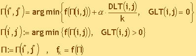
The first part is the determination of the best
solution in the N environment. First, a solution is sought according to the
formula (*) in such a way that the pair of elements (i, j) in the solution
vector is rearranged. The expression in braces is computed, the objective
function for the current solution vector is computed, a value equal to the
product of the penalty for frequent switching of the pair (i, j) and the
frequency of switching the pair (i, j) is added to this value. These
operations are performed to shift the pair (i, j) from the entire
environment. The environment is all possible adjustments, ie those for which
the grace period T = 0. The pair whose adjustment gave the smallest value of
the expression in brackets (*) is remembered. Then a solution is sought
according to the expression (**). This time, the environment are all changes
for which the grace period is greater than zero. The value of the objective
function is computed for each implementation of the shift (i, j) from the
environment N. If the solution found by the expression is better, it is taken
as the best solution found in step k. Then a memory correction is performed.
The grace period for pairs for which switching is prohibited is reduced by 1.
For the pair whose switching gave the best solution in step k, the grace
period T on the Upper Tabu List is substituted and the counter of the
occurrence of switching this pair on the Lower Tabu List is increased by 1 in
the process of finding the best solution.
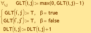
The Tabou list can be realized with a square matrix
with a dimension equal to the size of the problem under study, but references
to elements on the main diagonal of the matrix are not allowed for a simple
reason - the matrix remembers the permutation (rearrangement) of two
different elements. It is difficult to talk about a permutation of the same
element. The figure below shows the implementation of short-term (GLT) and
long-term (DLT) memory using matrices. This is an example of a problem with
the dimension n = 9, grace period T = 5, and the situation on the Tabu List
is presented after iteration, in which the elements (5,8) were switched.
The lower part of the DLT matrix contains the long
term memory. It remembers all the changes of pairs of elements, after each
switching of a pair of elements, it increases the memory cell for this pair
by 1. The pair (3,2) has already been switched 3 times, pairs (4,1), (7,1),
(9,1 ), (8,2), (9,7) only once, etc. The main diagonal of the matrix is not available. |
||||||||||||||||||||||||||||||||||||||||||||||||||||||||||||||||||||||||||||||||||||||||||||||||||||
|
|
||||||||||||||||||||||||||||||||||||||||||||||||||||||||||||||||||||||||||||||||||||||||||||||||||||
|
A frequently considered example of the application
of the QAP model is the location of production plants (machines in the plant
hall), where the set N defines a set of localities (set of positions in the
hall) where plants (machines) should be built (set up). In this case, the
matrix A is a matrix of distances between locations (positions), while the
matrix of relations B=[bij] describes the mutual dependence of plants or the
flow of materials (parts) between the plant (machine) j and l. The linear
component, described by the matrix C=[cij] can be interpreted as the cost of
building the plant j in the locality i.
|
||||||||||||||||||||||||||||||||||||||||||||||||||||||||||||||||||||||||||||||||||||||||||||||||||||
|
|
||||||||||||||||||||||||||||||||||||||||||||||||||||||||||||||||||||||||||||||||||||||||||||||||||||
|
|
||||||||||||||||||||||||||||||||||||||||||||||||||||||||||||||||||||||||||||||||||||||||||||||||||||
|
The QAP problem research program based on the Tabu
Search algorithm was written in a Windows environment using Borland
International's Bilder C ++ version 4.0 utility, as the name suggests in the C
++ object-oriented programming language. The project is called Krzyś and
consists of 7 files: executable file krzys.exe, project source file
krzys.cpp, files containing individual classes vector.h, table.h, TS.h,
QAP.h, files with windows forms Mform.h, Aform.h and the corresponding files
of the same name with the extension .cpp, containing implementations of class
member functions. A detailed description of the classes is provided below. |
||||||||||||||||||||||||||||||||||||||||||||||||||||||||||||||||||||||||||||||||||||||||||||||||||||
|
Figure 1. Appearance of the toolbar with buttons. The first button from the left
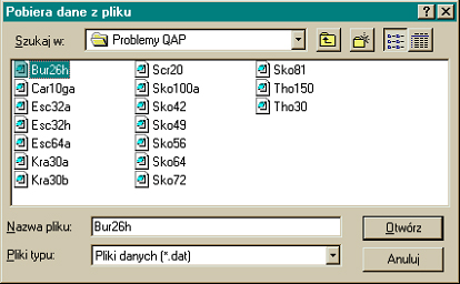
"Otwórz" allows you to load the problem from the file. Pressing the
button opens a dialog box that allows you to browse directories and files on
disks and select a data file to open.
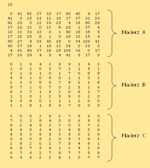
Figure 2. Dialog box for opening data file. Data files should have the following structure: The first number to read from the file should be the
problem size, then the next numbers are the elements of matrix A, then the
elements of matrix B, and possibly the elements of matrix C. Pressing the OK
button closes the file open dialog box and if the file format is inconsistent
with the one presented above, the program will report the error: "Incorrect file format". On
the other hand, if the file structure is correct, the data will be loaded
into appropriate table variables, the main program window will enlarge and
will look like it is shown in the figure below.
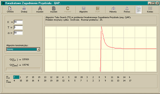
Figure 3. Program window appearance after opening a data file. At the top there is a description field that
contains information about the file from which the problem was loaded and its
size. "Tabu Search (TS) algorithm in
the Quadratic Assignment Problem (QAP). Problem loaded from file ............
dat. The size of the problem: ...."
On the top left there is a field for setting
algorithm parameters. There are three edit fields here that allow you to
enter new values. The first field allows you to change the number of K
iterations at which the algorithm stops. The second field allows you to
change the value of the grace period for a given pair T, i.e. the number
entered specifies the number of iterations through which the replaced pair
cannot be changed in search of a better solution. The third edit field gives
the possibility to change the parameter a, which is a penalty incurred by the
pair for having already been changed in the process of searching for a better
solution. Below is a drop-down list that allows you to select
a construction algorithm to derive the Pst start solution. There are three algorithms on the list: random,
algorithm 1, algorithm 2. The first determines the vector of the starting
solution using a random number generator. The second and third work as
described in section 1.2.2 of the Best_Match procedure. Algorithm 1 sums
successive elements in individual rows of matrix B, orders the sums in a
non-ascending order and creates a vector BB from them, then sums the
successive elements of columns in matrix A, orders the sums non-decreasingly
and creates vector AA from them, and then constructs the starting solution
vector assigning successive elements vector BB to vector AA elements.
Algorithm 2 works on the same principle, but differs in that it sums the
elements in individual columns of matrix B, arranges the sums in
non-ascending order, sums the elements in successive rows of matrix A, orders
the sums in non-decreasing order, the vector of the starting solution is
constructed in the same way as the Algorithm 1. Underneath is an algorithm progress indicator that
shows how many iterations have been done. At the bottom there is a field in which the starting
and minimum solution vectors are displayed. These are all the necessary
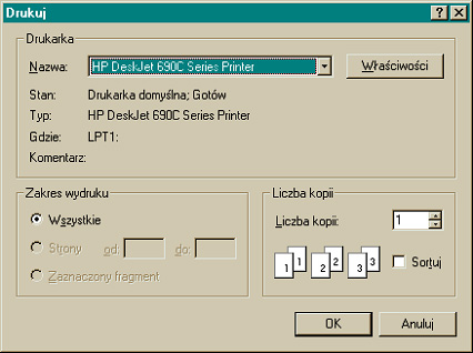
elements in the window for efficient operation of the algorithm. The next button on the toolbar is the Print button.
Pressing this button will open the printing dialog box as shown in the figure
below.
Figure 4. Print dialog box. The printing dialog box displays the current status
of the printer, its name, and allows you to open the printer properties
window, where, depending on the type and software of the printer, you can
perform, among others, changes in paper quality, print quality, and many
other options; has a field to enter the number of copies for printing.
Pressing the OK button causes the current program window to be printed. The
next three buttons allow you to preview the matrix with data, i.e. pressing
the Matrix A button displays the data in matrix A in the program window,
similarly the buttons Matrix B and Matrix C.
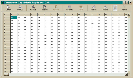
Figure 5. The appearance of the program window after pressing the
Matrix A button. The next Algorithm button displays the algorithm
window described above in the description of the Open button. Another Start button
runs the Tabu Search algorithm and is active only when the algorithm window
is visible. After pressing the button, the course of the objective function
is drawn on the graph, the current value of the objective function is
displayed on the left, and the algorithm progress indicator changes below the
number of iterations until the number of iterations reaches the value of the
K parameter.
Figure 6. Program window appearance after the algorithm completes
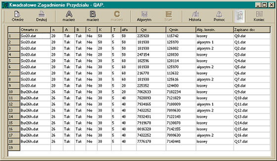
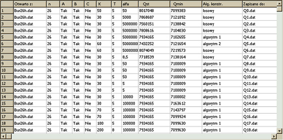
calculations. The History button
displays a window with all the algorithm calls, i.e. the window contains a
list where a new record is added each time the algorithm is called. The
record contains the following information about a given algorithm invocation:
file where the data comes from, problem size, whether the problem contains
matrix A or matrix B or matrix C, values of parameters K, T and alpha, value
of the start and minimum target function, file to which successive values of
the objective function were saved while searching for a solution.
Figure 7. Program window appearance after pressing the History button. The
next Help button displays the program help. The program help contains basic
information about the QAP problem and the Tabu Search procedure as well as
the program's manual. The last button available is the End button, which ends
the program. The toolbar also contains a drop-down menu that can
be called by right-clicking within the toolbar.
Figure 8. The appearance of the drop-down menu for the toolbar. Using
the drop-down menu, you can decide what is to be visible in the program
window. Ie. you can display the program's main menu, which is normally
invisible, you can disable the button bar or only the button labels, you can
enable or disable the main window display, you can enable or disable the
display of the status bar. The status bar contains hints or information about
the object currently under the mouse pointer. When the status bar is
invisible, the same information is displayed in the algorithm window above
the graph. The main menu contains the same options as the buttons on the
toolbar. Additionally, you can display the program card with basic
information about the program and the author. These are all basic information
about using the program. The next section presents in detail how the graphic
interface was implemented and describes in detail the functions of handling
individual events, e.g. pressing a button. |
||||||||||||||||||||||||||||||||||||||||||||||||||||||||||||||||||||||||||||||||||||||||||||||||||||
|
|
||||||||||||||||||||||||||||||||||||||||||||||||||||||||||||||||||||||||||||||||||||||||||||||||||||
|
|
||||||||||||||||||||||||||||||||||||||||||||||||||||||||||||||||||||||||||||||||||||||||||||||||||||
|
|
||||||||||||||||||||||||||||||||||||||||||||||||||||||||||||||||||||||||||||||||||||||||||||||||||||
|
void
__fastcall TMainForm::OnCreate(TObject *Sender) Listing 1. The main form's OnCreate event handler function. In
the first line of the function, the OnHint event handler of the main form is
assigned the function of the same name OnHint. The OnHint event is generated
when the mouse cursor is moved over a component and displays a tooltip if one
has been previously defined for that component. By default, the hints are
displayed in the status bar and you do not need to define your own function
for handling the OnHint event. The program decided to display the tooltips
using the LabelOpisTS label belonging to the TabSheetTS page when the status
bar is invisible. The following is the contents of the OnHint function. void
__fastcall TMainForm::OnHint(TObject *Sender) Listing 2. The main form's OnHint event handler function. If
the status bar is not visible, display hints with the LabelOpisTS label.
Otherwise display them in the status bar. In
the second line of the OnCreate function, theOpis Historii function is called
to display the column labels in the StringGridHistoria component on the
TabSheetHistoria page. Below is the content of this feature. void TMainForm::OpisHistorii(void) Listing 3. OpisHistorii()
function. In the third line of the OnCreate
function, the global variable ileTS is reset, which counts the successive
calls of the Tabu Search algorithm, i.e. the next press of the Start button.
It was introduced to automatically number files to which successive values of
the objective function are written during the algorithm's calculations. The main menu commands have the same
event handling functions as the buttons on the toolbar. The Open button has
the operation function shown below. void __fastcall TMainForm::MenuOpenClick(TObject *Sender) Listing 4. MenuOpenClick() function. The first line declares an integer variable named
size, which is a local variable of this function and its task is to remember
the size of the loaded problem. On the second line, the open file dialog is
called. The ability to open the file has been limited to files with the .dat
extension by entering an appropriate filter in the filter property of the
dialog box component. If you click Cancel, no statements are executed and the
MenuOpenClick() function ends. If the data file is selected and the OK button
is clicked the rest of the statement is executed. A file object of the
ifstream class is created and the file with the name stored in the FileName
property of the file open dialog box is automatically opened. Since the
constructor of the file object of the ifstream class requires the char*
pointer type parameter, and the FileName property is an object of the
AnsiString class, the standard c_str() method was used, which ensures the
appropriate conversion. Then the first number from the file is read, which
informs about the size of the problem defined in the file. Next it is checked
whether the global variable pProblem, which is a QAP pointer, contains the
address of the object. If so, the object is destroyed and the pointer is
reset to zero. Then, memory is dynamically allocated for the QAP type object
with the address entered under the pProblem pointer, using the new operator.
The constructor of the QAP class is invoked with one parameter in which the
problem size is passed. The next line calls the WczytajMacierze(file)
function of the QAP object to read the data from the file. A detailed
description of the functions can be found later in the work, when individual
classes are discussed in detail. The WczytajMacierze function returns the
number of matrices read from the file. It is used in the following lines to
set bool variables MatrixA, MatrixB, MatrixC, QAP object to true or false,
respectively, and depending on which matrices have been read, the appropriate
buttons on the toolbar are blocked. Previously, ButtonActivate(true) is called, which
makes all buttons active. When the function parameter is false, all buttons
are blocked. void TMainForm::ButtonActivate(bool _aktywne) Listing 5. ButtonActivate(bool _aktywne) function. Then,
if the program view was limited to the toolbar, the program window is
enlarged and the TabSheetTS page of the PageControl component is displayed.
The next line checks if a TS object exists by checking whether the pTabu
pointer contains the address of the object or the value of NULL. If the TS
object existed, it is destroyed and the pointer is reset to zero. Then memory
is dynamically allocated for the TS object, using the new operator, the
constructor of the TS class is called, and the address of the object in memory
is assigned under the pTabu variable. The next line updates the problem
information with the LabelOpisProblemu on the TabSheetTS page. The name of
the data file and the size of the problem are changed. The Repaint() method
ensures that the new data is displayed correctly. The following lines reset
the data in the StringGridPI component that displays the starting and minimum
solution vectors. Also the content of the graph is cleared. This is ensured
by the following lines. Then the "Start" button is blocked until
the construction algorithm is selected and the starting solution is
determined. Then the "Start" button is made available. These are
all actions performed in the MenuOpenClick() function if the execution of the
WczytajMacierze(file) function was successful. Otherwise, the object with the
address stored under the pProblem indicator is deleted and a window with the
following information is displayed: Wrong file format! Finally, the file is
closed and the file object is destroyed. After executing the MenuOpenClick()
function, memory was allocated for two objects. The first object was created
on the basis of the QAP class containing data about the problem and the
second object was created on the basis of the TS class, prepared to handle
the TabuSearch algorithm. void __fastcall TMainForm::MenuPrintClick(TObject *Sender) Listing 6. MenuPrintClick() function. This
function only has one line where the print dialog is called. If the OK button
is pressed, the Print () method is called and causes the current window to be
printed. Depending on which page of the PageControl component is active, this
will be printed. The
buttons Matrix A, Matrix B, Matrix C have similar operating functions. void
__fastcall TMainForm::MenuAMatrixClick(TObject *Sender) Listing 7. MenuAMatrixClick() function. void
__fastcall TMainForm::MenuBMatrixClick(TObject *Sender) Listing 8. MenuBMatrixClick() function. void
__fastcall TMainForm::MenuCMatrixClick(TObject *Sender) Listing 9. MenuCMatrixClick() function. In
the first and second line of the function, the main program window is
activated if it was inactive. All the above functions differ in the third
row, in which the current page of the PageControl component is determined,
i.e. which matrix is to be displayed. The instruction on the last line
disables the Start button, which is activated only when a new construction
algorithm is selected. The
Algorithm button has the operation function shown below. void __fastcall TMainForm::ToolButtonTSClick(TObject *Sender) Listing 10. ToolButtonTSClick() function. The
function has only two lines, the instruction in the first turns on the main
program window if it was invisible, the instruction in the second sets the
active page of the PageControl component to TabSheetTS. The
Start button has the operation function shown below. void __fastcall TMainForm::ToolButtonStartClick(TObject *Sender) Listing 11. ToolButtonStartClick() function. In
the first part of the function, variables are declared: two integer
variables, the first named i used for indexing in the for loop, the second
named size, which is initialized with the value returned by the function ZwrocRozmiar()
of the QAP object; three objects of the String type, initialized with the
values of K, T, a parameters, and taken from the edit fields on
the TabSheetTS page; one Wektor object named Pii; two integer variables, k
storing the number of iterations, t storing the grace period value for a
given pair; one float variable named alpha that holds the value of the alpha
parameter. The statements following the try statement are then executed. If
execution of any of these statements fails, an exception will be thrown,
caught by the catch statement, and the exception handling statements will be
executed, ie a dialog will be displayed with the information: Invalid
parameter! This means catching an exception that the conversion cannot be
performed using StrToInt() or StrToFloat(). These conversions are performed
on the first lines following the try statement. Then the new k, t, alpha
parameters obtained after converting the text from the edit fields are
entered into the TS object using the functions defined for this object: NoweK(),
NoweT(), NoweAlfa(). The next line calls the TS object's AlgorithmTS()
function, which contains the body of the TabuSearch algorithm. This feature
will be discussed later in this work. After the TabuSearch algorithm
computes, the DodajDoHistorii() function is called. The program remembers
each invocation of the algorithm along with the parameters of its invocation,
and saves them as another record in the table on the TabSheetHistoria page.
This is what the DodajDoHistorii () function does. void TMainForm::DodajDoHistorii() Listing 12. DodajDoHistorii() function. The first line declares three objects a, b, c of the
String class. Then, depending on the contents of the variables MacierzA,
MacierzB, MacierzC, QAP object, objects a, b, c are assigned strings Yes or
No. Then, for the current record, individual values are entered
into the subsequent columns of the table. In the first field of the record,
the name of the file from which the data comes is entered, in the second
field the problem size n previously obtained using the ZwrocRozmiar()
function of the QAP object. In the next three fields, the contents of the
objects a, b, c are entered, the next three fields contain the values
of the parameters K, T, a retrieved from the TS object using
the functions ZwrocK(), ZwrocT(), ZwrocAlfa(),the next two fields are the
values of the start and minimum objective function, also retrieved from the
TS object using the functions ZwrocQst() and ZwrocQmin(). The next field is
filled with a string returned by the function ZwrocAlgorytmSt() of the QAP
object, the last field of the record contains the name of the file where the
next values of the objective function have been stored, this
name is entered using the ZwrocNazwePliku() function of the TS object. In the
penultimate row of the DodajDoHistorii() function, a new record is created in
the StringGridHistory table and numbered with the next value in the last row. In the next line of the ToolButtonStartClick ()
function, the local Pii object of the Wektor class is assigned the solution
vector obtained after the execution of the AlgorytmTS() function. The
solution vector is obtained from the TS object using the function ZwrocPImin().
In the following lines the vector Pii is entered into the StringGridPI table.
Then the page content is refreshed, and the value of the objective function
calculated for the found solution is displayed using the LabelQmin label,
namely its Caption property. void
__fastcall TMainForm::ToolButtonHistoriaClick(TObject
*Sender) Listing 13. ToolButtonHistoriaClick() function. The
function displays the main program window if it was invisible, switches the
active page in the PageControl component to TabSheetHistoria and blocks the
Start button. The
End button has the operation function shown below. void __fastcall TMainForm::MenuExitClick(TObject *Sender) Listing 14. MenuExitClick()
function. The
function checks for the existence of QAP and TS objects. If so, they are
destroyed. The Terminate() method is then called to terminate the program. Above
are presented all operating functions defined for the toolbar buttons and the
same commands of the main menu. There are other events in the program that
have their own handling functions. These functions are outlined below. Clicking
the Matrices command from the main menu executes the operation function shown
below. void
__fastcall TMainForm::MenuMatricesClick(TObject *Sender) Listing 15. MenuMatricesClick() function. The function is to check, when you click the
Matrices of the main menu command, which page of the PageControl component is
active, and to set the marker in the drop-down menu for the Matrices of the
main menu to the appropriate position.
Figure 9. Matrices command in the main menu. The MenuWidokClick() function handles an event
related to selecting the View command in the main menu. The View command
manages the program view, ie it enables or disables individual program window
elements: toolbar, main menu, main program window (PageControl component),
status bar. The MenuWidokClick() function checks which items are visible when
the View command is selected, and on this basis update the markers next to
items visible or invisible in the expanded menu when the View command is
selected.
Figure 10. Main menu View command. void
__fastcall TMainForm::MenuWidokClick(TObject *Sender) Listing 16. MenuWidokClick() function. By
selecting the View command from the main menu, the MenuWidokClick () function
is performed and the submenu shown in Figure 10 is expanded. Selecting the
Button Bar command performs the operation function shown below. void
__fastcall TMainForm::MenuPasekprzyciskowClick(TObject
*Sender) Listing 17. MenuPasekprzyciskowClick() function. This
function enables or disables the visibility of the second band of the CoolBar
component on which the bar with buttons was placed. In addition, the function
has a protection against switching off the button bar when the main menu is
invisible. In this case, the function automatically enables the visibility of
the main menu, and more precisely the first band (indexing from 0) of the
CoolBar component. The
function MenuMenuglowneClick() below works similarly. void
__fastcall TMainForm::MenuMenuglowneClick(TObject *Sender) Listing 18. MenuMenuglowneClick() function. This
function is activated after selecting the Main menu command from the submenu
shown in Fig. 10. It enables or disables the visibility of the main menu, has
the same protection as the MenuPasekprzyciskowClick() button menu function. The
MenuOknodanychClick() function is performed when the Main window command is
selected from the submenu shown in Figure 10. Enables or disables the
visibility of the PageControl component. void
__fastcall TMainForm::MenuOknodanychClick(TObject *Sender) Listing 19. MenuOknodanychClick() function. The
MenuPasekstatusowyClick() function is performed when the StatusBar command is
selected from the submenu shown in Figure 10. Enables or disables visibility
of the StatusBar component.
void
__fastcall TMainForm::MenuPasekstatusowyClick(TObject
*Sender) Listing 20. MenuPasekstatusowyClick() function. The MenuTekstnaprzyciskachClick() is
designed to enable or disable text labels on toolbar buttons. void
__fastcall TMainForm::MenuTekstnaprzyciskachClick(TObject
*Sender) Listing 21. MenuTekstnaprzyciskachClick() function. The
above function, additionally, after disabling the display of text labels on
the buttons, changes the size of the buttons. The size of the toolbar is
automatically adjusted to the size of the buttons by setting its AutoSize
property to true. The
StatusBarDblClick () function has a handler function as shown below. void __fastcall TMainForm::StatusBarDblClick(TObject *Sender) Listing 22. StatusBarDblClick() function. This
function is to disable the visibility of the status bar after double-clicking
the right mouse button in the area of the bar. The
ComboBoxClick () function is called when an item is selected from the
drop-down list on the TabSheetTS page. There are three items on the list, the
names of the available construction algorithms. Selecting an item from the
list by clicking it with the left mouse button causes the event handling
function which is presented below. void __fastcall TMainForm::ComboBoxClick(TObject *Sender) Listing 23. ComboBoxClick() function. The
function above in the first line declares two local variables of integer type,
the first one named i used as an index in a for loop, the second the size
initialized on the same line with the value returned by the ZwrocRozmiar()
function of the QAP object. The second line declares a local object called
alg of the String class, initialized with the text selected from the ComboBox
drop-down list, the third line declares a local object of the Wektor class
named Pii. Next, the QAP Object AlgorytmStartowy function is called with the
alg parameter. This function contains three algorithms that generate a
startup solution, the appropriate algorithm is called depending on the alg
parameter. A detailed description of this function is presented later in the
work, during the description of functions and components of objects. |
||||||||||||||||||||||||||||||||||||||||||||||||||||||||||||||||||||||||||||||||||||||||||||||||||||
|
|
||||||||||||||||||||||||||||||||||||||||||||||||||||||||||||||||||||||||||||||||||||||||||||||||||||
|
class Wektor Listing 24. Wektor class. Private
fields of a class are an integer pwektor pointer that stores the address of
an area in memory reserved for the created object of this class, and an
integer variable n that stores the size of the vector. The Wektor.h header
file shown in Listing 26 contains only the Wektor class structure. The exact
structure of the function, i.e. its implementation, can be found in the
Wektor.cpp file. Only the construction of a function constructing objects of
the Wektor type is presented below. Wektor::Wektor(int
_n) Listing 25. The
Wektor class constructor. In
the first line of the function, memory is dynamically allocated for an array
of integer elements with the dimensions passed to the function by the _n
parameter. The address of the memory area is written to the pwektor variable.
In the second line of the function, a private variable of class n is
initialized with the value passed by the _n parameter. In the next two lines,
a Wektor object is initialized to 0 using a for loop. |
||||||||||||||||||||||||||||||||||||||||||||||||||||||||||||||||||||||||||||||||||||||||||||||||||||
|
|
||||||||||||||||||||||||||||||||||||||||||||||||||||||||||||||||||||||||||||||||||||||||||||||||||||
|
The Tablica class was created in order to construct
square matrix objects with integer elements. This class has two private
fields, an integer ptab pointer to the memory area where memory is allocated
for a two-dimensional array, and an integer variable n that stores the size
of the matrix. The class has three constructors, a destructor, and overloaded
assignment operators and function calls. Like the Wektor class described
above. The structure of the Tablica class is shown below. class Tablica Listing 26. Tablica class. The
above structure is a class header file named Tablica.h. On the other hand,
the function definitions, ie the structure, are in the file Tablica.cpp. Only
the construction of the Tablica class constructor is shown below. Tablica::Tablica(int
_n) Listing 27. The Tablica class
constructor. In
the first line, the new operator dynamically allocates memory for an integer
array of pointers of the size given in the parameter to the _n function. The
memory address where the pointer table is stored is entered under the
variable ptab. Then, with the for loop, memory is allocated for the array of
integer elements, and in each iteration, the address of the allocated memory
area is written to the next element from the previously dynamically created
pointer array. The next two for loops initialize the array elements with the
values of 0. In the last line of the function, the size stored in the local
variable _n is copied to the private variable of the object named n. |
||||||||||||||||||||||||||||||||||||||||||||||||||||||||||||||||||||||||||||||||||||||||||||||||||||
|
|
||||||||||||||||||||||||||||||||||||||||||||||||||||||||||||||||||||||||||||||||||||||||||||||||||||
|
class QAP Listing 28. QAP class. The
class has five private fields, the first is an integer variable size that
stores the size of the problem this object concerns. The next three fields
are Tablica class objects used to store the matrices read from the file that
define the current problem. The next field is an object of the Wektor class
that stores the solution vector. This vector changes during the operation of
the Tabu Search algorithm due to the replacement of individual pairs of
vector P elements. The last field is the AlgStartowy object of the String
class that stores the name of the startup algorithm selected from the list.
The first public member function is a constructor with one parameter to pass
the size of the problem. This function calls the constructors of the Tablica
and Wektor classes directly and assigns the created objects to private
objects of the QAP class. The function WczytajMacierze() is to
read data from a file and write them under private objects A, B, C. { Listing 29. WczytajMacierze() function. In
the first line of the function, all characters in the file are counted by the
while statement. This action is to find out how many matrices with data are
in the file. A properly defined problem has two or three matrices. The
program exits the loop when it encounters an end-of-file character. In the
second line of the function, the file pointer is placed at the beginning of
the file. Then the first number from the file, which is the problem size, is
read. This information is not needed for this function and is not used. Data
download starts with the second number. Depending on the number of counted
numbers in the file, i.e. on the value of the variable number ile, numbers
are read successively and entered as successive elements of private objects
A, B, C. Depending on the number of defined matrices in the file, the
function returns the number of read matrices. The
AlgorytmStartowy(String) function is to create a startup solution, i.e. the
vector of the startup solution. Depending on the parameter passed to the
function, the startup solution is generated using one of the three available
algorithms. bool QAP::AlgorytmStartowy(String _alg) Listing 30. AlgorytmStartowy() - losowy function. When
the parameter of the function is a sequence of characters 'losowy', the starting
solution is generated based on the randomization of successive elements of
the vector. The algorithm works in such a way that it randomizes a number, if
it is the first drawn number, it enters it as the first element of the
starting solution vector. If it is another number drawn, the algorithm checks
whether such a number has already been drawn. If the vector already contains
such an element, a new draw is performed until a number different from all
the vector elements drawn so far is obtained. If
the algorithm parameter is a sequence of characters 'algorytm 1', the
starting solution is generated on the basis of the list serialization method
described in section 1.2.2. The following is a continuation of the AlgorytmStartowy(String)
function. else
if(_alg
== "algorytm 1"){ Listing 31. AlgorytmStartowy() - algorytm1
function. In
the first two lines, memory is dynamically allocated for an array of
Para-type structures and the address of the allocated memory area is written
under the pointer variables rA and rB. Each pair contains two fields. In this
case, the first field i of the pair rA were used to store the sum of the
elements in individual lines, the second field is the line number. The first
two for loops do the summation of items across lines. The sums are then
sorted in ascending order using the qsort function from the BilderC ++
standard library Stdlib. The last for loop generates the start solution
vector in such a way that the minimum value of the field i of the pair rA is
assigned to the maximum value of the field i of the pair rB. This averages
the value of the objective function, and thus the optimal solution is found
faster. In the same loop, the memory for the structure tables rA and rB is
released. If
the parameter of the function is the sequence of characters 'algorytm 2' then
the vector of the starting solution is generated based on the algorithm shown
below. else if(_alg == "algorytm 2"){ Listing 32.AlgorytmStartowy() - algorytm2 function. The
above algorithm differs from the one in Listing 31 only in that it counts the
sums of the elements of the individual columns of matrices A and B, not the
rows. If the matrices are symmetric, the vector of the starting solution
generated by Algorithm 1 is the same as the vector generated by Algorithm 2. The
function WypiszMacierze() is called inside the WczytajMacierze() function to
display matrices A, B, and C on the appropriate pages of the PageControl
component. At the beginning, the function determines the page properties -
StringGrid components: ColCount sets the number of columns (the value is
greater than the size of the problem by one column because the first column
contains individual row numbers), RowCount determines the number of rows (the
value is greater than the size of the problem because the first row contains
the numbers of each columns), Cells[0][0] is the upper-left corner element of
the StringGrid component and contains the name of the matrix. Then the rows
and columns of the matrix are numbered, and the values of matrices A, B and C
are entered under individual Cells[i][j] elements of the StringGrid
components. void QAP::WypiszMacierze(void) Listing 33. WypiszMacierze() function. The
Permutation (Para &p) function is designed to switch two elements (passed
as a parameter) in the solution vector P. The function has one local variable
used to store one element of the pair passed as a parameter. This is
necessary to properly swap two items. void
QAP::Permutacja(Para &p) Listing 34. Permutacja() function. The function Q() calculates the value
of the objective function. Its structure is presented below. double QAP::Q(void)
Listing 35. Q() function. The
above function declares two local variables of the double type, which hold
the sums of the auxiliary objective functions. The first one contains the sum
calculated by adding the appropriate elements of matrix C, the second one
contains the sum calculated by adding individual products of the elements of
matrices A and B. The function contains two local integer variables serving
as indices in the for loop. The
QAP class contains still various functions for accessing its private fields.
They enable saving new values from the outside or reading the current values
of individual fields. An example would be the ZwrocRozmiar() function, which
returns the value of a private variable size. int QAP::ZwrocRozmiar(void) Listing 36. ZwrocRozmiar() function. |
||||||||||||||||||||||||||||||||||||||||||||||||||||||||||||||||||||||||||||||||||||||||||||||||||||
|
|
||||||||||||||||||||||||||||||||||||||||||||||||||||||||||||||||||||||||||||||||||||||||||||||||||||
|
The TS class was created in order to construct
objects that are designed to perform and store data about the Tabu Search
algorithm. The class has 11 private fields, two of the integer type: K holds
the number of iterations, T holds the grace period (blocking) value for a
given pair; one alpha floating point field holds the value of the parameter
which is a penalty for frequent pairing; LT object of the Tablica class,
which is a tabu list for the Tabu Search algorithm; pointer QAP Problem that
stores the address of the object where the QAP problem is defined; two objects
PImin, PIst of the Wektor class holding the start and minimum vectors; two
variables Qst, Qmin of the double type holding the values of the start and
minimum objective function; an AnsiString NazwaPliku object that stores the
filename for storing the value of the objective function; object Plik of ofstream
class to provide a write operation to the file. class TS Listing 37. TS class. The
class has one constructor with a parameter where the address of the object
where the QAP problem is defined is passed. The function UstalProblem() is to
initialize three private fields of TS class. Its structure is presented
below. void TS::UstalProblem(void) Listing 38. UstalProblem() function. The
private object PIst is initialized with the boot solution vector obtained
from the QAP object through the public function ZwrocPI() of the QAP class.
Private variable Qst is initialized with the value of the objective function
computed by the public function Q() available in the class QAP. The private
variable Qmin is initialized with the value of the variable Qst, because the
minimum value of the objective function is initially the starting value. The
AlgorytmTS() function is to determine the best solution to the problem
defined in the QAP object, using the Tabu Search algorithm. bool TS::AlgorytmTS(void) Listing 39. AlgorytmTS() function - local variable declarations. The
first part of the function is shown above. One integer variable k containing
the number of the current iteration is declared, two variables of the bool
type are declared: NoweQprim with the value true if the found current value
of the objective function is determined on the basis of the Qprim formula;
NoweQminodQprim() true when a new minimum value of the Qmin objective
function based on the formula Qprim is found; three gwiazdka, prim, loop
structures of the Para type to remember the pair of rearranged elements, i.e.
the gwiazdka remembers a pair of elements after the change of which there was
an improvement in the value of the objective function calculated by means of
the formula Qgwiazdka, prim remembers
a pair of elements after the change of which there was an improvement in the
value of the objective function calculated by means of the formula Qprim,
loop serves as a helper pair used in for loops. In the further part, three
local variables of the double type are declared to store the values of the objective functions
Qakt, Qprim, Qgwiazdka. Next, an integer variable rozmiar is declared,
initialized with the problem size value from the QAP object. Then the maximum
value of the progress indicator is set to the value of the K variable. In the next line, the file name is created
with the next number obtained from the ileTS global variable, and the file
with this name is opened for writing, where the value of the start objective
function is saved, and the count of algorithm calls is increased. for(k=1; k<(K+1); k++){ > <-- początek pętli głównej Listing 40. AlgorytmTS() function - visualization. In
the next part, the algorithm runs in the for loop. The number of iterations
is equal to the value of the variable K. The first five lines of the loop are
responsible for visualizing the solution search process on the TabSheetTS
page of the PageControl component. The value of the progress indicator is
changed to a value stored in the variable k, then the value of the objective
function is plotted in the graph window, and displayed using the LabelQmin
label.
Qprim
= Problem->Q(); Listing 41. AlgorytmTS() function - determining the best solution in
the environment. The
first part of the algorithm, according to its structure described in point
1.3 of the paper, concerns the determination of the best solution in the
environment. This is done by the part of the algorithm presented in Listing
43. The variable Qprim is initialized with the value of the objective function.
The variable Qgwiazdka has the same value, because in the first iteration
each element of the tabu list has the value zero, so the value of the second
term of the formula is equal to zero. The next operations take place in two
for loops, which are designed to switch in pairs all elements of the solution
vector using the Permutacja() function and after each conversion, calculate
the current value of the objective function using the Q() function of the QAP
class object. Then, two conditions specified in step 2 of the algorithm
described in point 1.3 are checked, and implemented by the if/else if loop.
If there has been an improvement in the value of the objective function, then
a pair of elements is remembered, after changing which the value of the
objective function has improved. If there has been an improvement in the
value of the objective function Qgwiazdka, then the asterisk pair is
remembered, if there has been an improvement in Qprim value, then the prim
pair is remembered. At the end of each iteration, the pivoted items return to
their starting position. The rest of the algorithm is presented below (step
3), in which the solutions are improved. Problem->Permutacja(gwiazdka); Listing 42. AlgorytmTS() function - improvement of solutions. By
means of the Permutacja() function, two elements stored in the variable gwiazdka
are displayed. Then the value of the objective function is calculated and if
it is better than the current minimum value, the solution vector is stored in
the PImin variable. Then the moved elements return to their position. If
there is a change in the value of the objective function Qprim, the current
value of the objective function is calculated after rearranging the elements
stored in the variable prime, and if it is better than the current value of
Qmin, the new solution vector is stored in the variable PImin. Then the moved
elements return to their position. The last part of the algorithm is
presented below, in which the memory state is corrected, i.e. the tabu list
content is updated.
for(loop.i=0;loop.i Listing 43. AlgorytmTS() function - memory state correction. Two
for loops are searched at the top of the tabu list and the value of each item
in the top tabu list greater than zero is decreased by one. Ie. the blocking
period for a given pair in each iteration is decreased by one. The tabu list
is then further revised using the if else statement. If the improvement of
solutions resulted from shifting a pair of prim elements (if statement), then
the position on the upper taboo list for these elements is initialized with
the value of the T parameter, this is the grace period for a given pair,
which is entered using the edit field on the TabSheetTS page; two elements in
the solution vector are shifted with the Permutacja() function of the QAP
class object; it is increased by one value of the lower tabu list for prim
pair elements, i.e. the counter of the occurrence of a given pair is
increased by one. If the solution was improved as a result of rearranging the
elements of the gwiazdka pair, the operations described above are performed,
but for the gwiazdka pair (the else statement). The last instruction in the
main loop of the algorithm writes the current value of the objective function
to a file. When the counter in the main for loop reaches the value of K, the
execution of the statements in the loop is terminated, and thus the Tabu
Search algorithm is over. The AlgorytmTS() function in the last three lines
closes the file for writing, sets the algorithm progress indicator to zero,
and returns true. |
||||||||||||||||||||||||||||||||||||||||||||||||||||||||||||||||||||||||||||||||||||||||||||||||||||
|
|
||||||||||||||||||||||||||||||||||||||||||||||||||||||||||||||||||||||||||||||||||||||||||||||||||||
|
The Para structure was created in order to remember
two integer elements. It has two public fields i and j, a function that
constructs a new object of the Para structure and initializes its fields with
zero values, an overloaded assignment operator that ensures the correct
assignment of one structure of type Para to another, the structure also has a
friend function of PorownajPary() to sort an array of Para structures in the
AlgorytmStartowy() function of the QAP class. struct Para Listing 44. Para structure. The
PorownajPary() function compares two pair structures according to the field
and the structures. Returns positive if the structure passed in the first
parameter to the function has a greater value in the field i than the
structure passed in the second parameter, or the function returns negative if
the field i of structure passed in the first parameter have a value smaller
than the field i of structure passed in the second parameter to the function.
int PorownajPary(const void
*arg1, const void *arg2) Listing 45. PorownajPary() function. |
||||||||||||||||||||||||||||||||||||||||||||||||||||||||||||||||||||||||||||||||||||||||||||||||||||
|
|
||||||||||||||||||||||||||||||||||||||||||||||||||||||||||||||||||||||||||||||||||||||||||||||||||||
|
The process of examining QAP problems using the Tabu
Search algorithm is presented below. Standard problems defined in files available
on the Internet were successively loaded into the written program. For each
problem, many series of tests were performed, changing the values of the
parameters K, T and Alpha and the Starting Algorithms. The created tool was
designed in such a way that after pressing one button on the toolbar, the
results can be obtained in a readable form in a table containing both the
minimum value of the objective function found, as well as the algorithm
invocation parameters and the defined QAP problem under investigation. Each
entry in the table shows the next performed test - a new Tabu Search
procedure call.
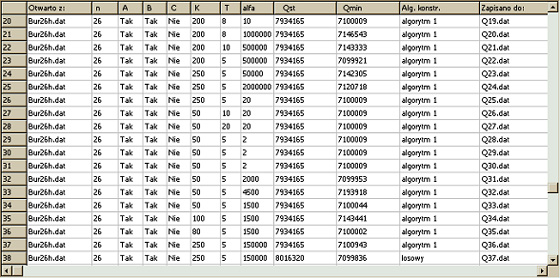
Table 1. Test results of studying the Bur26h problem of 26 size.
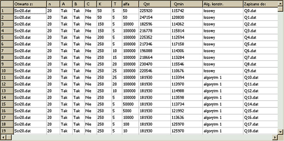
Table 2. The results of studying the scr20 problem of size 20.
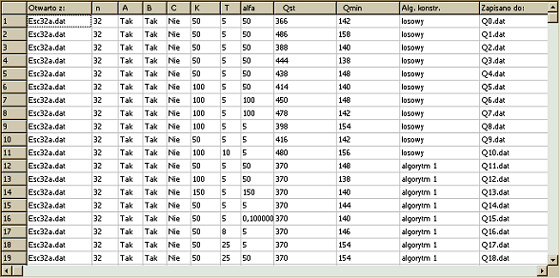
Table 3. Test results of studying the Esc32 problem of size 32.
Table 4. The results of the study of the size 32 Esc32h problem.
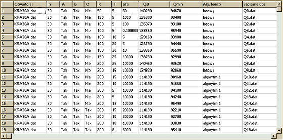
Table 5. The results of studying the Kra30a problem of size 30.
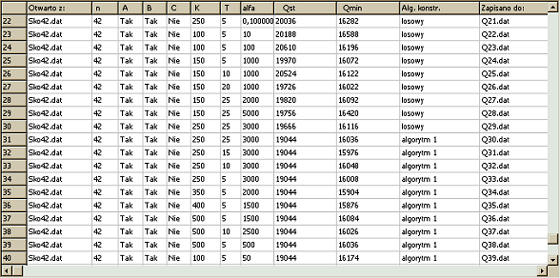
Table 6. The results of studying the Sko42 problem of size 42.
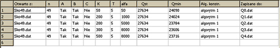
Table 7. The results of studying the Sko49 problem of size 49.
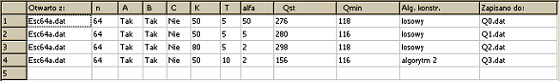
Table 8. The results of studying the Esc64 problem of size 64. |
||||||||||||||||||||||||||||||||||||||||||||||||||||||||||||||||||||||||||||||||||||||||||||||||||||
|
|
||||||||||||||||||||||||||||||||||||||||||||||||||||||||||||||||||||||||||||||||||||||||||||||||||||
|
Many standard data problems with files ending in
".dat" have been investigated. In the process of searching for the
best solution, the values of the T parameter and the Alpha parameter were
changed. The starting solution was generated on the basis of three different
algorithms, including one random and two averaging the initial value of the
objective function built on the basis of the BEST-MATCH procedure. The number
of iterations was also changed. The course of the objective function values in the
process of searching for the best solution to the Sko42 problem of size 42 is
presented below. K = 250 and Alpha = 3000 remained unchanged.
Chart 1. Examination of the Sko42 problem for T = 25, 15, 10 and 5 as
well as K = 250 and Alpha = 3000. As can be seen from the above diagram, the change of
the T parameter has an impact on the search for a solution in the Quadratic
Assignment Problem using the Tabu Search algorithm. For T = 25 the minimum
value of the objective function is 16036, for T = 15 the found value of the
objective function for the best solution is 15576, for T = 10 Qmin = 16048,
for T = 5 Qmin = 16008. As you can see, this parameter is used to
differentiate the search process the best solution in the Tabu Search
algorithm. The second parameter that was changed while testing the algorithm
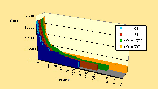
was the Alpha parameter. The graph below shows the curves of the objective
function values for different values of the Alpha parameter.
Chart 2. Examination of the Sko42 problem for T = 5 and Alpha = 500,
1500, 2500 and 3000. The Alpha parameter is a penalty for frequently
rearranging a pair of elements in the process of finding the best solution.
It was noticed from the above chart that when the penalty is small, the
algorithm quickly goes to a certain minimum, but it is not a satisfactory
solution. When the penalty was increased to 1500, it was found that the
algorithm is slower towards the minimum, and in this case the solution found
is better than when the penalty was 500. Further increasing the penalty, a
similar effect of slowly going to the minimum was observed. In the last case,
when the penalty is 3000, far too few iterations were used. The best solution
was found for a penalty of 1500. For all cases, the grace period for a given
couple was 5. Many series of tests were made for many problems of
the Quadratic Assignment Problem defined in matrix form. The program written
in the Bilder C ++ environment works correctly, and the implemented Tabu
Search algorithm minimizes the value of the objective function and finds an
approximate solution depending on the entered parameters K, T and Alpha. In order to find the optimal solution to a given
problem, it is necessary to perform many series of tests, changing the values
of the algorithm parameters experimentally, because each problem requires
different parameter values to find the best solution. |
||||||||||||||||||||||||||||||||||||||||||||||||||||||||||||||||||||||||||||||||||||||||||||||||||||
|
|
||||||||||||||||||||||||||||||||||||||||||||||||||||||||||||||||||||||||||||||||||||||||||||||||||||
|
|
||||||||||||||||||||||||||||||||||||||||||||||||||||||||||||||||||||||||||||||||||||||||||||||||||||
|
|